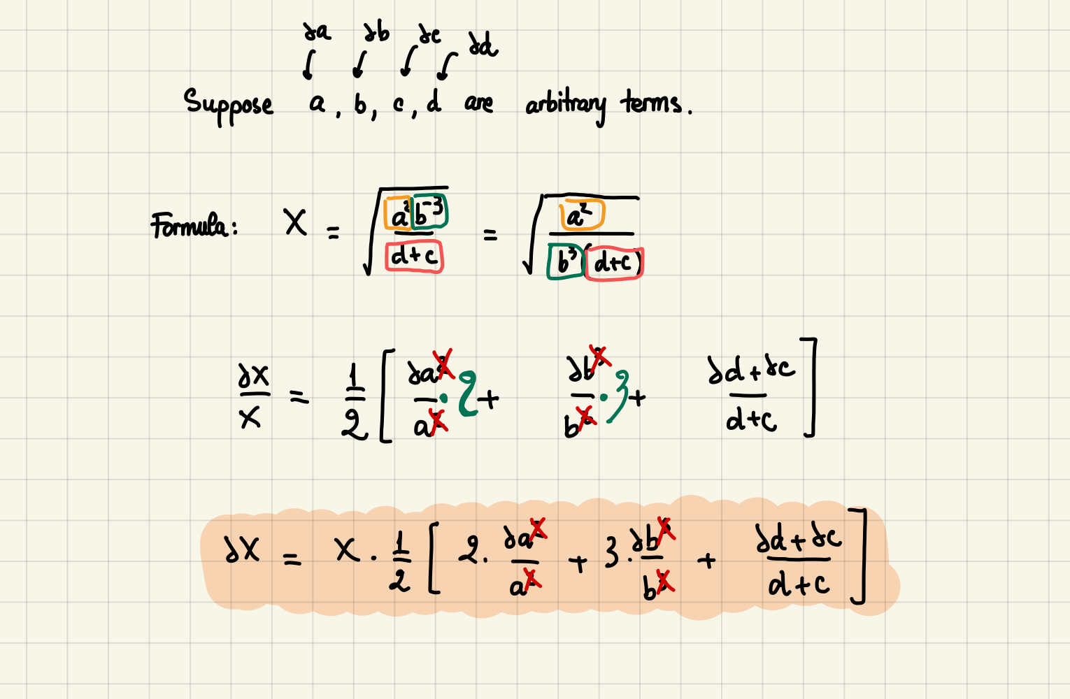
Lab 7
Here are some stuffs for lab 7!
Overview
This lab is an analogous experiment with Ohm Law experiment of Lab 6.
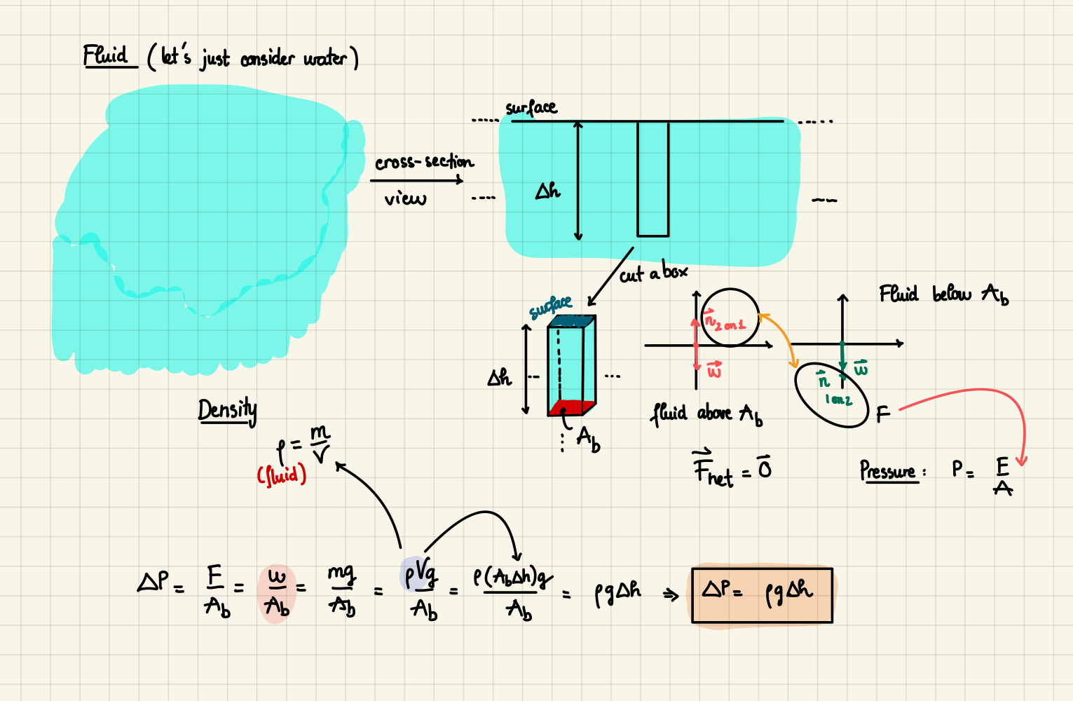
Some concepts are related to fluid dynamics. So, you might want to revise that topic.
Excel sheet will do all the works! Hopefully, it turns out quick for you.
Analogous relationship with electrical circuit
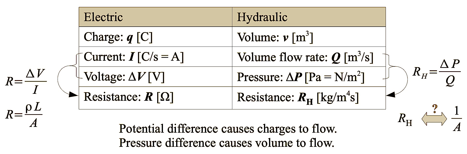
Fig. 26 Comparison with electrical circuit
Note
The setup is not a complete circuit as the fluid does not flow back to the other terminal.
Tables of known quantities
Name |
\(L(m)\) |
\(d_s(mm)\) |
\(d_m(mm)\) |
\(d_l(mm)\) |
\(\Delta{h}(cm)\) |
\(\rho(\frac{kg}{m^3})\) |
|---|---|---|---|---|---|---|
Value |
\(0.95\pm0.01\) |
\(0.28\pm10\)% |
\(0.64\pm10\)% |
\(0.99\pm10\)% |
\(23.1\pm0.5\) |
\(997\pm0\) |
Caution
Make sure to keep track your units! Do not mix them up!
Part 1: Data Collection & Calculation
In this lab, you are given 3 Youtube Videos for extracting data.
Note that the length of first video will be 31 minutes. And the others are approximately 5 minutes each.
Let’s take a look at the setup first:
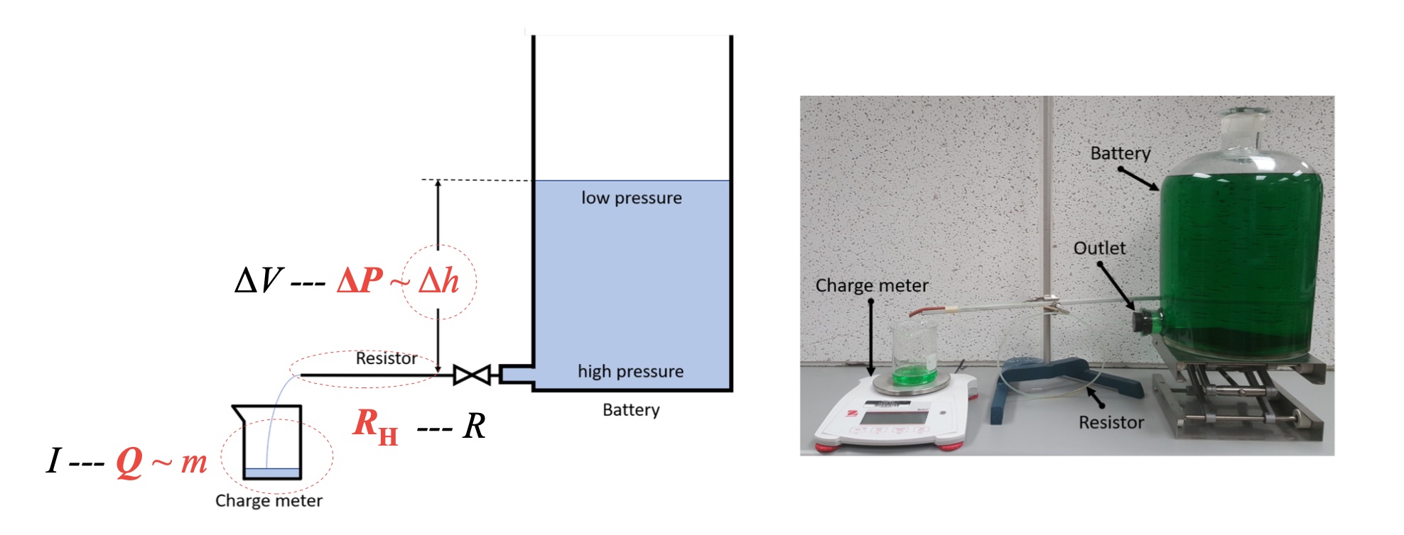
Fig. 27 Experimental setup
Section 1: Collection
Now, which pieces of information we are trying to extract? Mass value from the scale.
In each video, you need to find at least 12 values of mass. That means:
Choose 12 moments in the video.
Record the time. E.g. Time = 140s.
Record the scale reading according to each time.
Repeat the same pattern for the other two videos.
Tip
For the first video (small diameter), choose any moment as long as you gather at least 12 of them. For the other two, you can start from 20s and increment the time by 20s.
Section 2: Calculation
For the first 3 graphs, you need to find the Volume from Mass. How? Use \(\rho = \frac{m}{V}\).
For the last graph, there are several things to calculate:
\(\Delta{P}\): Find the pressure difference from \(\Delta{P} = \rho g \Delta{h}\)
\(Q\): Find the volume flow rate from the slope.
\(R_h\): Find the resistant of the tube from \(R_h = \frac{\Delta{P}}{Q}\)
\(A^{-1}\): Find the inverse of cross-section area of the tube. Not the battery/container.
Attention
All calculations must come with error calculations!
Part 2: Plotting
Now, there are 4 graphs you need to complete and submit.
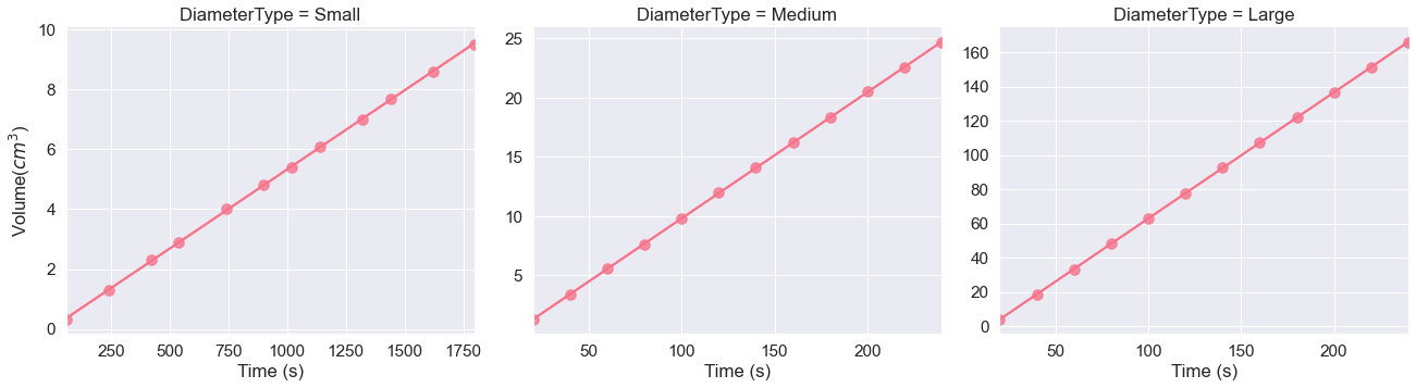
Graph 1,2,3: Plot Volume V (\(cm^3\)) vs Time (s).
Graph 4: Plot \(R_h\) vs \(A^{-1}\).
Attention
If you use \(cm^3\), please make sure to convert \(\rho\) to approriate unit.
Here is a demo for graph 1,2, and 3 for you to follow:
# Plotting
import pandas as pd
import numpy as np
import seaborn as sns
import matplotlib.pyplot as plt

# Read in data
dic = {1:"Small",2:"Medium",3:"Large"}
l = list()
for i in range(1,5):
    l.append(pd.read_csv(f"../../data/graph{i}_lab7.csv", delimiter="\t").assign(DiameterType=dic[i] if i < 4 else np.nan))

d4= l.pop()
df = pd.concat(l,axis=0)

# Initialize plots
sns.set_theme(style="darkgrid",font_scale=1.4,palette="husl")

# Plotting
g = sns.lmplot(y=r"volume(cm^3)",
               x=r"Time (s)",
               data=df,
               col="DiameterType",
               sharex=False,
               sharey=False,
               aspect=1.2,scatter_kws={"s": 90}
          )
g.set_ylabels(r"Volume($cm^3$)")
# Remove spine
sns.despine()

# Show plot
plt.show()
Attention
In your excel sheet, make sure to show equation with slopes, \({\bf R^2}\), and result of LINEST FUNCTION.
Here is another demo for the last graph:
# Ignore warnings for not enought data (not safe)
import warnings
warnings.filterwarnings('ignore')
fig = plt.figure(figsize=(8,6))
plot4 = sns.regplot(y="Rh (kg/m^4)",
                    x="A^-1 (m^2)",
                    data=d4,
                    order=2,
                    scatter_kws={"s": 90}
                   )
plot4.set(title=r"$R_h\ vs\ A^{-1}$",xlabel=r"$A^{-1}\ (m^2)$",ylabel=r"$R_h\ (\frac{kg}{m^4})$")
plt.show()
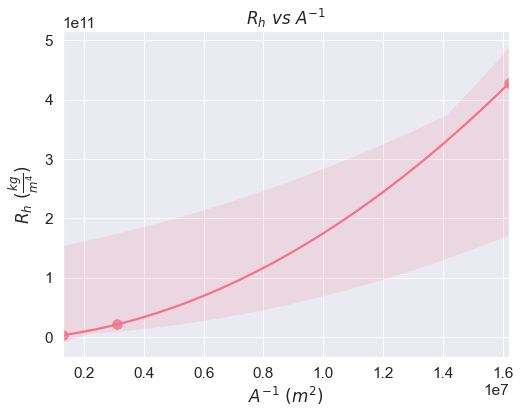
Tip
For this graph, choose fit line to power instead of linear (Excel). Then, extract the power component.
Discussion
Does plotting \(R\) vs \(A^{-1}\) remind you of lab 6? What did we analyze?
Basically, you want to see if they form a linear relationship as in electrical circuits (\(R = \rho \frac{L}{A}\)).
Which power is consider linear?