Lab 6
Here are some stuffs for lab 6!
Overview
This lab is probably the easiest and shortest lab so far.
Only error calculations are the majority of the work.
It requires a look-up for mapping resistivity and material type.
Plotting is required for submission.
Part 1: Calculations
Let’s have a look at the setup first:
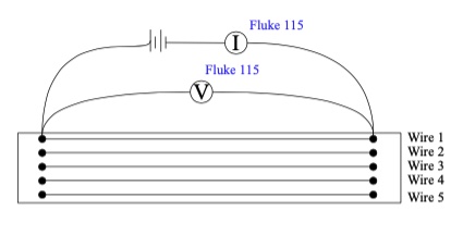
Fig. 24 Exmperimental setup
Your task is to collect values of \(V\), and \(I\) from the figures in lab manual.
There are 5 wires of increasing diameter of the same material corresponding to 5 figures. so, make sure to keep track on the figure label.
Next, you need to calculate other quantities such as:
Caution
The lab uses \(V\) as a replacement for \(\Delta{V}\) as we assume \(V_0\) = 0. Instead, \(\Delta{V}\) represents its uncertainty.
Uncertainty Calculations
Now, the manual says there is a special error measurement for \(\Delta{V}\) and \(I\).
Quantity |
Error Specifications |
|---|---|
\(\Delta{V}\) |
0.5% of the reading plus 2 digits |
\(\Delta{I}\) |
1% of the reading plus 3 digits |
Note
Those ‘2’ and ‘3’ digits are added to the last decimal places. The number of decimal places depends on your references. For the lab, three are enough.
Let’s have an example. You have found \(V = 9.321 V\). So its error is:
Note that we add 0.002 because we choose to keep 3 decimal place.
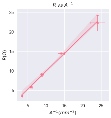
Part 2: Plotting \(R\) vs \(A^{-1}\)
Once you have all data ready, extract the R and x columns for plotting.
Now, you have 2 choices:
Logger Pro: Same steps as lab 1-5.
Excel: Use Scatter Plot with column R and x.
Attention
Make sure to add errors in the graph for either method!
Here is a demo for you to follow:
import matplotlib.pyplot as plt
import pandas as pd
import seaborn as sns

# Loading data set
df = pd.read_csv("../../data/lab6.csv", delimiter=",")

# Setting for plot
sns.set_theme("notebook", style="darkgrid", font_scale=1.3)
sns.set_palette("husl", 5)
plot = sns.lmplot(x="x",
                  y="R",
                  data=df,
                  scatter_kws={'s':70, 'edgecolor':'w'})
plot.despine()
plot.set_axis_labels(r"$A^{-1} (mm^{-2})$",r"$R (\Omega)$")
plot.ax.set_title(r"$R\ vs\ A^{-1}$")

# Now plot the error bar
plot.ax.errorbar(x=df["x"], y=df["R"], xerr=df["x error"], yerr=df["R error"], fmt='none', capsize=4)

# Show plot
plt.show()
Discussion
One question asks you to identify the wire material. This requires resistivity table to do the look-up.
Last question asks you to evaluate the relationship between R and \(A^{-1}\). Either use \(R^2\) (Excel) or Slope to justify your claim.
Tip
For resistivity, be careful as some metal is in form of liquid at room temperature!