Lab 5
Here are some stuffs for Lab 5!
Overview
This lab might seem a little too long but eventually it is not that bad.
You need an image editor to annotate your screenshots. E.g. Paint, Preview, PS.
We will need to plot 2 graphs from LoggerPro.
Excel work will start this week.
Attention
Please read the instructions in the manual on how to use the simulator!
Part 1: The Electric Dipole
Here, you need place 2 opposite charges on 2 halves of the surface (one left and one right).
Then, use the device with the cross-hair to draw the equipotential lines. How? Click the pencil.
Make sure you follow the required steps (not necessarily exact). In this case, it is \(\pm3(V)\).
Then, you need to draw Electric field Lines given the equipotential lines.
Here a demo for you to follow:
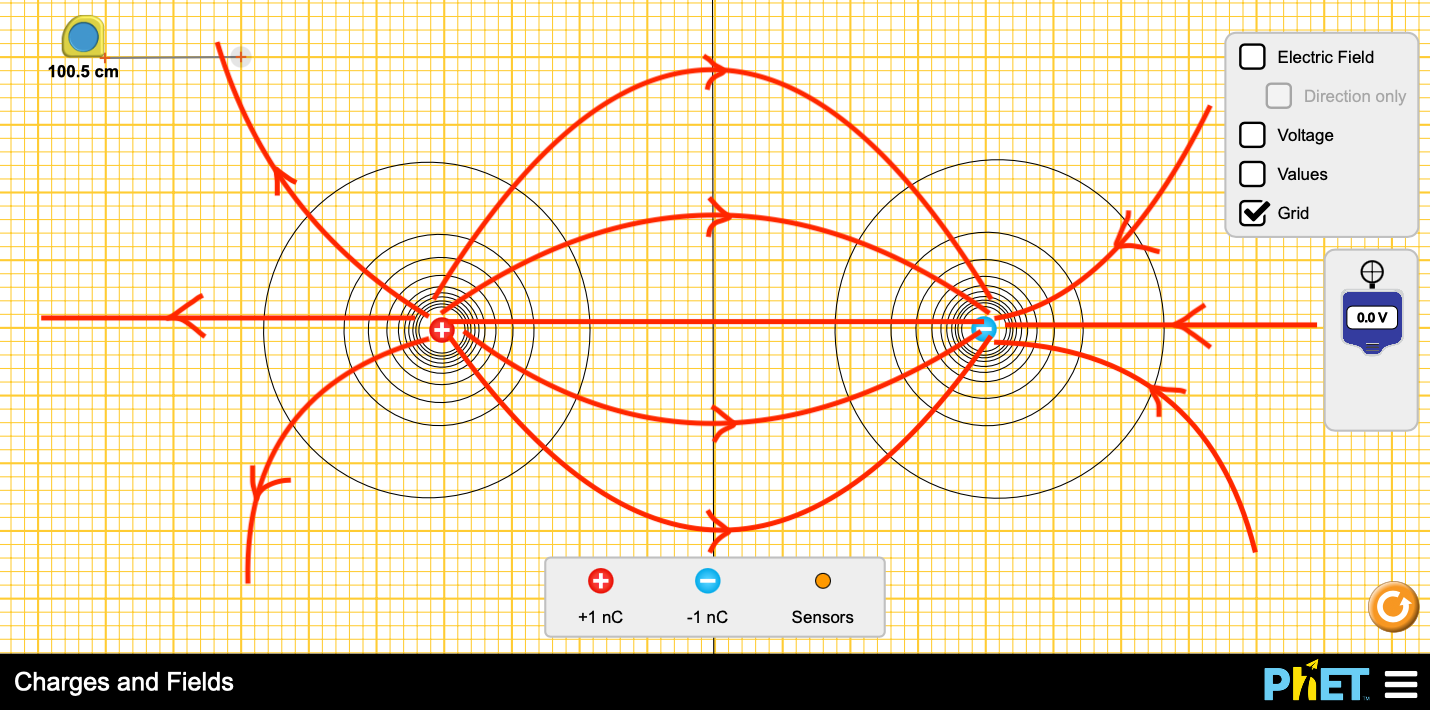
Fig. 18 Electric Dipole Simulation
Warning
Every image contains metadata, including author and created date. So, I would know whether you did it or copied somewhere.
Part 2: Pair of Like Charges
The procedure is similar to part 1. The only difference is that you place 2 same charges on 2 halves of the surface.
Make sure you follow the required steps (not necessarily exact). In this case, it is \(\pm1(V)\).
Then, draw the Electric field lines. Here is a demo for you:
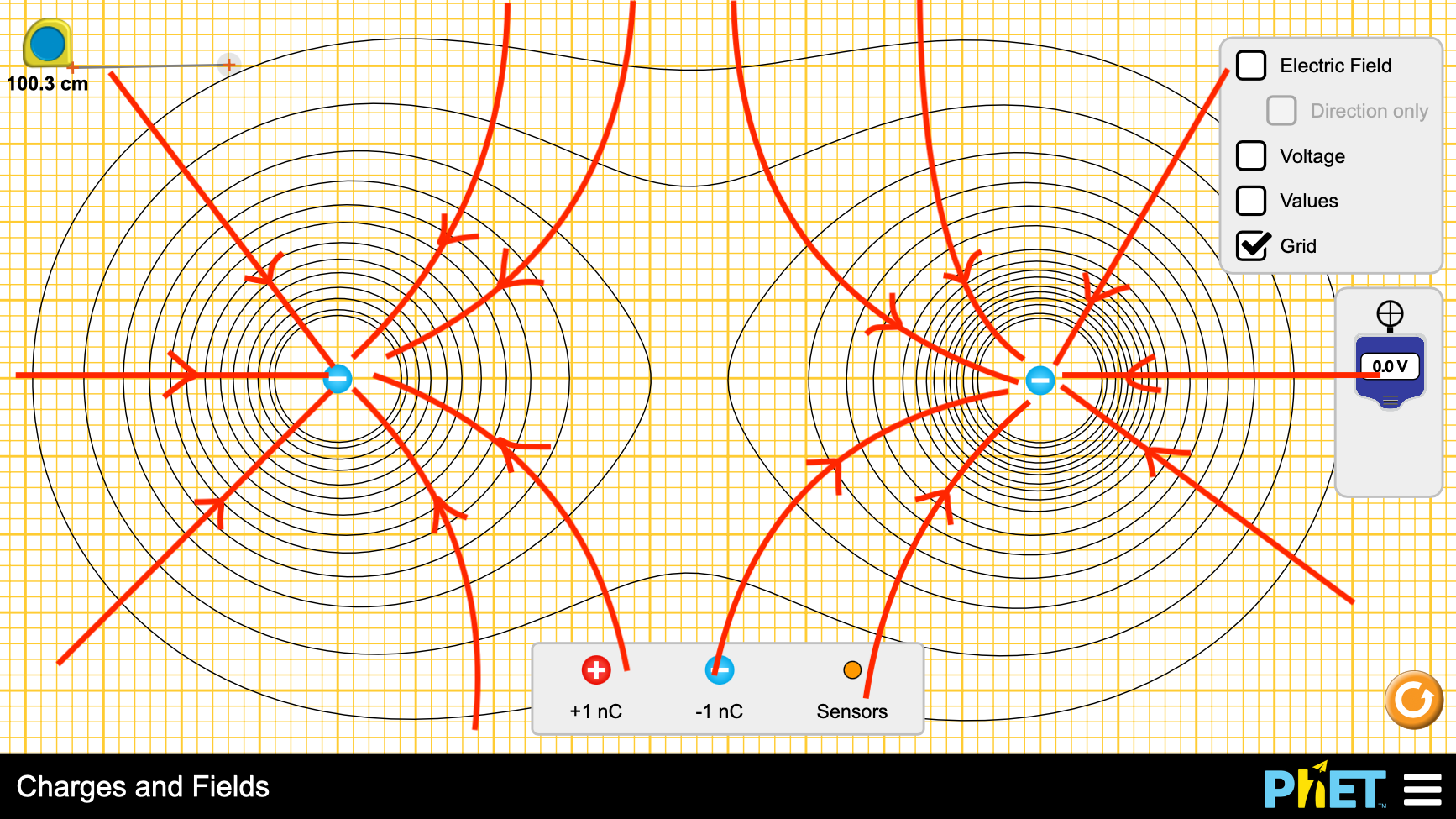
Fig. 19 Like charges simulations
Caution
Here, we have 2 like-charges. So be careful with the direction of the electric field lines.
Part 3: A Line of Charge
This part requires you to assemble a line of charges. Make sure to fill the entire browswer length.
Then, section 2 requires readings from cross-haired device and section 3 requries a sensor.
See also
Filling the entire length ensures that it behaves like a line of charges. Otherwise, some discrepancies might happen.
Here is demo of the setup for you to follow:
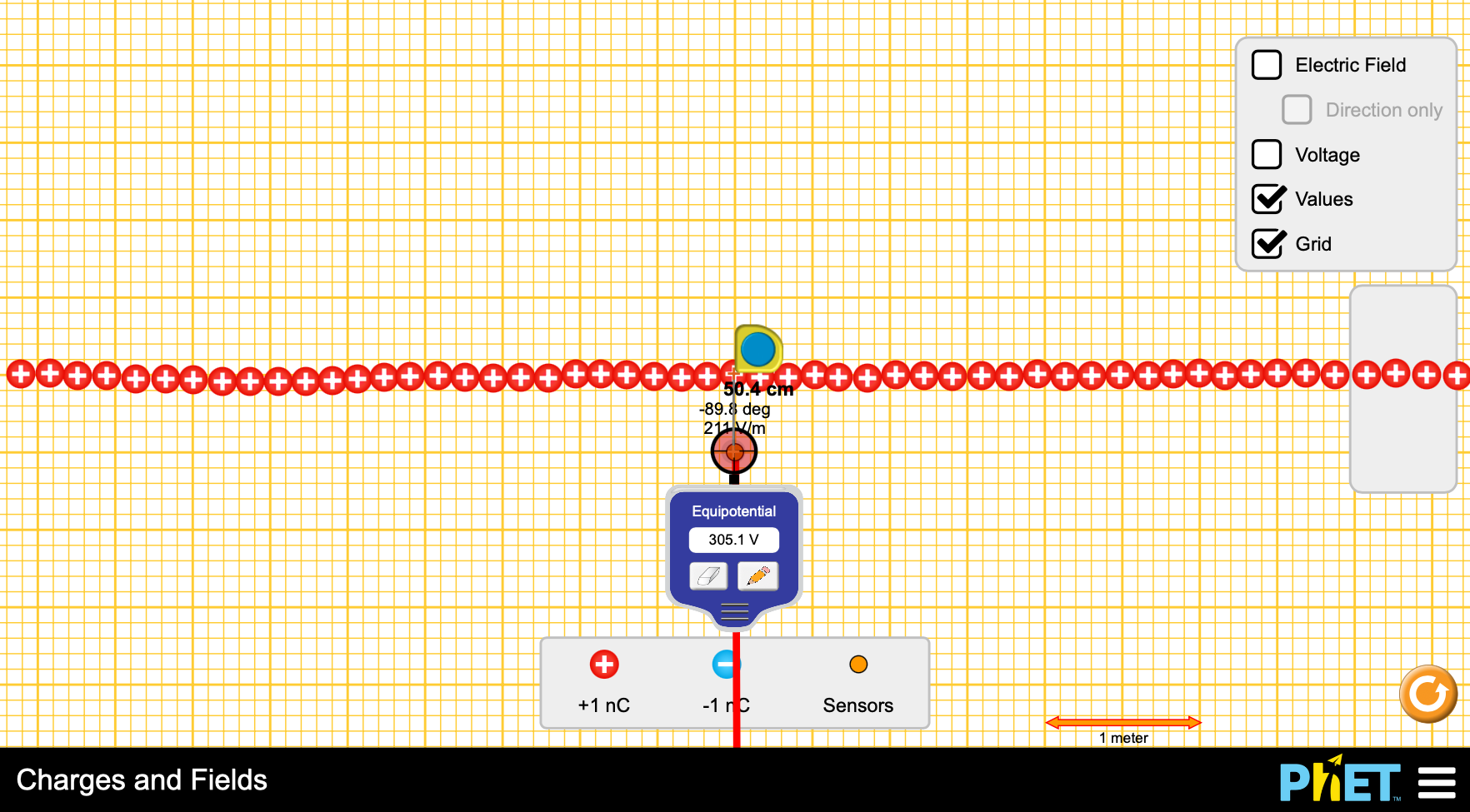
Fig. 20 Line of same charges
Section 1: Find the charge per unit length λ
You have the equation:
where:
n (number of charges).
q (charge per point)
L (length of line).
Tip
q is given in the simulator! Find it! Use nC or C.
So, you need to keep track on how many points you put in. Also, to find the length of the line, use the scale with the plus symbol at the tip.
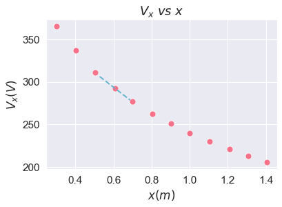
Section 2: Find estimated eletrical field strength Ex (V/m) at a point
Remember: We analyze at the middle of the line.
What you need to collect data is simple:
Step 1: Using the scale to find the distance x from the line midpoint. Starting from 0.1m with step of 0.1m.
Step 2: Use the crossed-hair device to read the potential Vx at that point.
Step 3: Record distance x and Vx in Logger Pro.
Step 4: Repeat until your you gather at least 12 points.
Caution
Tagent tool is interactive, so it only show the currently selected point.
After data collection, you need to:
Step 1: Use tagent tool to find slope at all points!
Step 2: Choose a point (Example: x = 0.605m).
Step 3: Go back to your simulator and place a sensor at that distance from midpoint.
Step 4: Read the value of Ex from the sensor and compare it to the slope.
Caution
Reading from sensor gave absolute values of Ex.
Here is a demo for Part 3 section 3:
import pandas as pd
import seaborn as sns
import numpy as np
import matplotlib.pyplot as plt

# Loading dada
part3_2 = (pd.read_csv("../../data/part3_2_lab5.csv", delimiter=",", dtype=float)
             .rename(columns={"x(m)":"x", "Vx(V)":"Vx"})
          )
part3_3 = (pd.read_csv("../../data/part3_3_lab5.csv", delimiter=",", dtype=float)
             .rename(columns={"1/x(1/m)":"1/x", "Ex(V/m)":"Ex"})
          )
# Settings
# Set seaborn themes
sns.set_theme(context='notebook',style='darkgrid', font_scale=1.4)
# sns.despine(left=True, bottom=True)
sns.set_palette("husl", 5)


# Plotting
plot = (sns.scatterplot(x="x", y="Vx",data=part3_2, legend = False, s=80,linewidths=0.7, edgecolor='w')
)
# Add title to only this subgraph
plot.set_title(r"$V_x\ vs\ x$", fontdict={'fontsize':18, 'fontweight':"bold", 'va':"baseline"})
plot.set_ylabel(r"$V_x (V)$")
plot.set_xlabel(r"$x (m)$")

# Choose a x
x = part3_2["x"][3] # Let's choose the third point
y = part3_2["Vx"][3]
upper = (part3_2["x"][2], part3_2["Vx"][2])
lower = (part3_2["x"][4], part3_2["Vx"][4])
# Define x data range for tangent line
xrange = np.linspace(x-0.08, x+0.08, 10)

def line(x,y, x_range, lower_neighbor, upper_neighbor,):
    slope = (upper_neighbor[1] - lower_neighbor[1])/ (upper_neighbor[0] - lower_neighbor[0])
    return slope*(x_range - x) + y

# Plot the tagent line
plt.plot(xrange, line(x, y, xrange, lower, upper), 'c--', linewidth = 2)
plt.show()
Section 3: Find estimated potential Vx (V) at a point
As you do section 2, you can also do section! Remember: We analyze at the middle of the line.
Repeat the same steps of data collection but you instead use sensors to read Vx and record x for calculating 1/x.
Once you are done, you need:
Step 1: Enter data into Logger Pro. Remember to use Ex and 1/x.
Step 2: Use linear fit tool.
Step 3: Extract the slope. Slope = Vx
Step 4: Show uncertainties
Now, compare the slope to your calculate Vx by extracting constant from this formula:
Tip
What does y axis represent and what does x axis represent? Also, \(\lambda\) is found in section 1.
Here is a demo for part 3 section 3:
plot2 = (sns.lmplot(x="1/x", y="Ex",data=part3_3, scatter_kws={'s':80, 'linewidth':0.7, 'edgecolor':'w'})
    .set_axis_labels(r"$\frac{1}{x} (\frac{1}{m})$",r"$E_x$ (V/m)")
)
# Add title to entire figure since we have only 1 plot
plot2.ax.set_title(r"$E_x\ vs\ \frac{1}{x}$", fontsize=18, fontweight="bold", va="baseline")
plt.show()
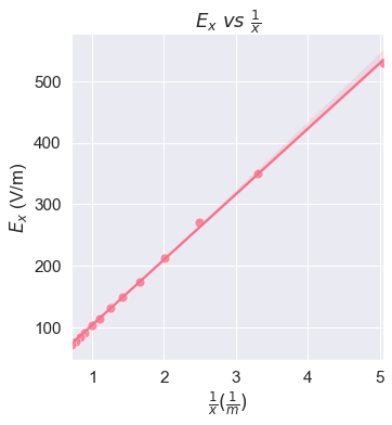
Caution
These graphs are not the actual graph you need to submit! Please use Logger Pro!
Discussion
We do not have a discussion part for this lab. But there are few things you need to remember.
There are several questions asking you to describe the pattern. So, please give your best observations. It must be your own.
Tip
One important concepts: The closer the equipotential lines are, the stronger the eletric field in those areas.
Excel Work (Closed)
Please keep track on the schedule. Rules must also be followed.
For lab 3, Click Here.
For lab 12, Click Here.
Excel Sheet
Lab 3 work: Click Here
Lab 12 work: Click Here
Note
Thank you everyone for your hard work! Hopefully, this allows you to learn to collaborate and practice Excel skills.